Benchmarking Quantum Computers vs Classical Computers

Originally published on Medium: benchmarking-quantum-vs-classical

---

Benchmarking Quantum Computers vs Classical Computers

When 11-year-old me learned about benchmarking, I wondered what on earth benches had to do with ranking computer performance.

Surely marking benches wasn’t a good thing. Isn’t that vandalism?!

That was before I watched Linus Tech Tips, where I understood that a “bench” is a common term used to describe a computer system being tested.

As for the term “marking”, that just refers to the computer’s performance reference, often marked on platforms such as, Geekbench, Cinebench and many others.

But that got me thinking, has anyone ever tried benchmarking a Quantum Computer before? I mean, surely it’s not as straightforward as benchmarking classical computers right?

So to find out more, I spent some time obsessively diving deep into the science and engineering of Quantum Measurements, and here’s what I have to say.

Benchmarking in Classical Systems

In the world of Classical Systems, like the phones and computers you and I both love, the three primary components benchmarked include CPUs, GPUs and Memory.

Often what these benchmarks measure is speed (which I’m grouping in with parallel performance)— which is extremely important for determining whether your system can run the software you want it to (looking at you Cyberpunk 2077), or will it just crash and burn.

What these benchmarking systems do is run your computer through a standardized series of tests, and rank them in comparison to thousands of other computer parts around the world.

Depending on the benchmark you’re using, the types of tests may vary quite a bit. One kind of test is called a Synthetic Benchmark, which looks at your computer’s performance on a series of hard operations like file compression, floating-point operations and so on.

The reason why it’s called a “Synthetic” benchmark is because they don’t actually run real-world applications. They are just simulating these hard operations.

On the other hand, Real-World Benchmarks actually test your computer components in real-world situations (like rendering graphics) to see how it performs — not every component uses the same metrics though!

Generally speaking, when your computer is under heavy load you will experience a decrease in performance. This decrease usually comes in the form of losing frames, decreased data throughput, render time and so on.

The better your component’s base speed is, and the heavier the load it can take before speed starts to drop, the better your component is.

The Formula

When talking about benchmarking Quantum Computers, it’s important to note a couple of fundamental differences in the way we evaluate the performance of these systems, compared to classical ones.

For starters, Quantum Computers don’t work quite like classical computers do. They are not standalone computers — far from it actually.

Almost every implementation of a Quantum Computer to date is hybrid. This means two things.

One, for a quantum computer to actually receive instructions from us and give them back to us in a form that we can understand, we must use classical computing equipment alongside the quantum computer.

And two, quantum computers are often used as parts of a bigger workflow, a component working as part of a bigger system.

What this means for benchmarking is that instead of looking at just the sheer speed of a quantum computer, we also need to look at the speed of its readouts, advanced control electronics, runtime and so much more.

Moreover, Quantum Computers work according to the fundamental laws of Quantum Mechanics. It’s a double-edged sword really — being able to do really complex calculations in a fraction of the time a classical computer would take, in return for errors, decoherence and a myriad of other issues stopping us from doing these computations in the first place!

In order for us to improve on these more fundamental aspects of quantum computing, we need to look at two other metrics as well: Scale and Quality.

Here’s a simple formula for you: Performance = Scale + Quality + Speed.

A trifecta of metrics, determining the performance of a quantum computer, corresponding with its overall “usefulness”.

The Pyramid

Back in what I believe was 2020, IBM first unveiled their first Benchmarking Pyramid, describing the kinds of possible benchmarks that can be done at different levels of a quantum system. Here’s what that looks like:

Re-themed version of IBM’s Pyramid

There are three core levels: Device, Subsystem and Holistic.

While IBM works on Superconducting Qubits as their quantum technology of choice, this can be applied to almost any quantum computing system.

Each level has an entirely different design, protocols, and metrics for success. As we go up the pyramid, the difficulty to interpret the entire system (including the levels below it) becomes way more complex.

The Device level looks at the design and related fabrication of qubits.

The Subsystem level looks at the calibration of the qubits.

And finally, the Holistic level looks at the entire system from a high-level, examining the compilation of circuits and the way they dynamically decouple.

Each of these metrics are interesting enough to deserve their own articles. So in interest of your time and sanity, I will be only be covering a select few metrics from the first two levels.

Device Level

Let’s examine T1 and T2 on the device-level — kudos to this simple and concise paper for the great explanation!

You might recognize the T1 and T2 from quantum circuit building. Each “T” refers to some time instant where gates are run.

However, these same characters also refer to two constants important for measuring quantum decoherence. For starters, T1 refers to Thermal Relaxation Time, theoretically defined as the time needed for a qubit to move from an excited state |1> to a ground state |0>.

This can be formulated by the following density matrix:

Here, ⍺ and β refer to the probability amplitudes of the states. This naturally means that ⍺² is the probability that the qubit is in the state |Ψ> while β² is the probability that the qubit is in the ground state |0>.

Experimentally, it’s a bit more complicated — it’s the time by which the number of excited states (their “population”) decays to 1/e of their initial value given by the following formula:

Let’s break this down. Your first question may be “Why/what is 1/e?”

You see, e is the base of natural logarithms approximately equal to 2.718.

The expression “1/e” is used commonly when discussing exponential decay processes of radioactive substances for example, as well as quantum state decay. It represents a natural and mathematically convenient way for processes where the rate of change of a quantity is proportional to the quantity itself.

This helps us to think about how a system’s population may decay (in this case, lose population) over a period of time.

Hence, another way to think about T1 is the time it takes for the excited states population to decay to 1/e, around 37% of its initial value!

Now, let’s have a closer look at the formula. P_e(t) represents the probability that the overall system is in the excited state at some time t.

The initial system’s state would be when the time is 0 — that’s exactly what P_e(0) represents.

Given these two expressions, we can now formulate the decay of P_e(0) (the initial system state) by multiplying it with the exponential decay factor of e^-t/T1.

Let’s graph this formula to see how it looks:

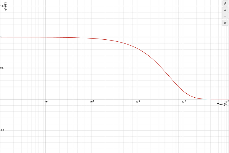
Here in this graph, I chose an arbitrary value of 50 microseconds (µs) for T1.

If you think about it, the ratio of t/T1 essentially determines how many multiples of T1 have passed since the process started. The larger the value of t/T1, the further the system has decayed.

If T1 = 50 µs, then after:

• 50 µs: The system will have a 37% chance of still being in the excited state.
• 100 µs: The system will have a 13.69% chance of still being in the excited state.
• 150 µs: The probability of the system remaining in the excited state is now just ~5%.

Keep in mind that T1 is a purely experimental value — there is no generalized formulation to derive it. Instead, it has to be carefully extracted in a lab environment.

As for the minus sign, that indicates that this quantity is decreasing over time. If we wanted to measure exponential rates of growth instead of decay, we would remove the minus sign.

T2 refers to Dephasing Time. While T1 is used to identify the time required for a qubit to move from its excited state to its ground state, T2 is defined as the amount of time it takes from start to finish (elapsed time) before a qubit’s resonance frequency (representing its coherence) becomes unidentifiable.

Resonance Frequency is defined as the frequency at which a quantum system (such as a qubit) naturally oscillates/vibrates. This allows is to absorb energy from certain external sources, allowing it to transition between energy levels easily.

This is quite a simple metric to measure. All you have to do is apply a Hadamard Gate, aka put the qubit in superposition, and then wait some arbitrary time t before sending another Hadamard Gate through to return it to its ground state.

When you measure the state of the qubit, you will be able to see a graph like so:

Source | A graph representing the Dephasing Time of a quantum device

Keep in mind that to actually measure these metrics on a real quantum computer, you will need access to Pulse-Level Control.

At the end of the day, both of these metrics are pivotal in quantifying noises and disturbances in quantum systems that prevent it from giving accurate results.

This is especially important as the scale of the number of qubits in a quantum system increases, introducing even more potential errors.

Subsystem Level

Let’s examine Randomized Benchmarking (RB) on the subsystem level.

Randomized Benchmarking is the standard way we measure and characterize gate errors on quantum computers.

There are two kinds of Randomized Benchmarking — 1-qubit and 2-qubit. Here we will just discuss the 1-qubit variant.

The goal here is to design a sequence of certain gates such that when the unitary is run, it leaves the system in exactly the same state as it was before (the identity operation).

While that may seem odd, the purpose here is to test the underlying hardware of the quantum computer based on the number of errors produced from the computation.

The error rates for the device are estimated based on how frequently the system returns to the correct state versus an error state, specifically the number of shots resulting in an error.

We use a standard circuit made up of randomized Clifford Gates to calculate this. Although a standard RB experiment provides gate errors for every Basis Gate (the simplest gates a quantum computer can process, meaning that every gate must be simplified to them), these gates can be added up to create a Clifford Gate — namely a Hadamard Gate, S Gate or CNOT Gate.

The circuit evaluates the overall error over a sequence of these Clifford Gates, producing an averaged Clifford Gate error.

It’s important to note that the more gates are applied, the more likely errors are to accumulate. Hence the RB method uses this trend to estimate the “mathematical trueness” (fidelity) of the system, based on the number of errors which in turn signifies the performance of the system. Fewer errors = Better system.

If you are keen to explore this further, I highly suggest you check out the two resources below (note that their Qiskit versions are now outdated):

Randomized Benchmarking - Qiskit Experiments 0.7.0
*Randomized benchmarking (RB) is a popular protocol for characterizing the error rate of quantum processors. An RB…*qiskit-community.github.io

textbook/notebooks/quantum-hardware/randomized-benchmarking.ipynb at main · Qiskit/textbook
*Source content for the Qiskit Textbook. Contribute to Qiskit/textbook development by creating an account on GitHub.*github.com

Quantum Benchmarking Software

I briefly want to go over some of the popular benchmarking software scientists have created over the years.

Each one has their own unique advantages and specifications. Here are some of the ones I came across (in no particular order):

• SoK: https://www.mdpi.com/1099-4300/24/10/1467
• QPACK — Using QAOA as a benchmark: https://arxiv.org/pdf/2103.17193
• BACQ — An application-oriented benchmark: https://arxiv.org/pdf/2403.12205

Some notable mentions include:

• MQT Bench — Benchmarking Software and Design Automation Tools: https://quantum-journal.org/papers/q-2023-07-20-1062/pdf/
• SupermarQ: A Scalable Quantum Benchmark Suite: https://ieeexplore.ieee.org/abstract/document/9773202
• QUARK — Framework for QC Application Benchmarking: https://arxiv.org/pdf/2202.03028

Of course, unless your paper is published in a top-tier journal, it’s not easy for people to notice your contributions to quantum benchmarking.

In fact, I’d argue that the whole format of publishing these benchmarks in papers across various journals makes it quite difficult to compare and contrast them.

Fortunately, the team over at Unitary Fund have created Metriq, a community-driven platform for doing exactly that — showcasing the performance of methods on platforms against tasks.

Methods are the algorithms, platforms are the hardware and tasks are the workloads used.

Conclusion

There has been a lot of discussion as to whether quantum computers are going to replace classical ones. But I would like to believe that they’re each meant for entirely different kinds of computations.

The fundamental way we examine metrics in a quantum system versus a classical one is quite different. There is so much more we have to take into account when talking about quantum systems, and we haven’t even got to looking at speed yet!

It’s not as simple as looking at a component or two. You have to get a holistic look at the entire architecture of the device instead.

That’s why I completely agree with IBM, with their claims about the future of quantum being “hybrid”.

I believe that these systems are meant to be used alongside classical computers, in order to do specialized things that they just aren’t capable of yet.

But what do you think? Let’s spark some engagement in the comments down below 👇👇