DNA Computing — the Quantum Computing Killer?

Originally published on Medium: dna-computing

---

DNA Computing — the Quantum Computing killer? 🎃🔪

An image generated by Dall-E3 on DNA Computing killing Quantum Computing on Halloween

I stumbled across this paper on DNA Computing a couple of days ago, and it instantly captivated my curiosity.

DNA Computers can perform parallel computations incredibly efficiently, making it possible to solve complex problems that regular computers would take an infeasible amount of time to solve.

But as it happens to be, Quantum Computers are often referred to as having this same computational characteristic. And so when I was done reading, I was left more so with a sense of dread rather than awe — “Is this the end of Quantum Computing?”

To answer this question, I decided to take a deep dive into the Theory of Computation, and this article is all about my findings!

Buckle up, and enjoy the read 🎢 📖

DNA Computers

DNA Computers were invented by Leonard Adleman in 1994. They are capable of performing massively parallel computational tasks using, you guessed it, DNA.

Unlike digital computers, which only utilize two bases to perform computations, DNA computers use four of them called nucleotides. They are A (Adenine), C (Cytosine), G (Guanine), and T (Thymine). This means that classical computers are base-2 systems, while DNA Computers are base-4 systems.

One of the things that makes them so great is their remarkable energy efficiency. You can theoretically execute 2x10¹⁹ operations per joule of energy on a DNA Computer. Compared to supercomputers of the 20th century, which topped out at just about 10⁹ operations per joule. That is literally the difference between the length of a meter stick and 952 Great Walls of China put together!

An image generated by Dall-E3 attempting to showcase the magnitude of 952 great walls of China put together in a spiral

Furthermore, DNA’s information storage density surpasses all known storage technologies by several orders of magnitude. The double-helix structure of DNA enables it to store vast information within a small form factor, approximately 1 bit per cubic nanometer. To put this in perspective, if every movie ever made were encoded in DNA, it would be smaller than a sugar cube!

Here is another image generated by Dall-E3 attempting to showcase the smallness of every movie ever created put into a sugar cube

This article describes how Adleman used this computer to solve the Traveling Salesman problem — the goal of which is to find the shortest route between a number of cities, where you can only go through each city once. As you add more cities to the mix, the problem becomes more and more complex, depending on the algorithm you’re using to solve the problem.

Here’s how he did it:

• He started off by using strands of DNA to represent each city and the possible paths that connect them together. There are a total of (n-1)!/2 solutions in the standard version of this problem, where n is the number of cities there are.
• In this case, he was working with 7 cities. That’s (7–1)!/2, or 360 possibilities.
• He then mixes the strands together in a test tube, allowing them to go through a process called hybridization.
• Hybridization is when DNA strands from different molecules like to stick to each other in a sequence, thereby undergoing a series of chemical reactions. This pairing process is individual, which is what makes these computers so good at parallel processing!
• Each chain of strands represents a possible answer, after which the wrong ones need to be eliminated using further chemical reactions.
• This leaves behind the optimal strands that connect all seven cities together!

If the series is right, hybridization will occur, outputting a “1” analogous to conventional computing. If it’s incorrect, hybridization will not occur, outputting a “0” in return.

While this experiment did produce optimal results, it took him days to filter out the sub-optimal combinations, which he had to do manually. The two biggest drawbacks of this technology at the moment? A lack of automation and speed.

If you’re a Quantum Computing enthusiast, you might have begun to notice some similarities between the two computing devices. To be able to compare and contrast the two computing technologies effectively, we need to learn about a little something called the Church Turing Thesis.

The Church Turing Thesis

Alan Turing was truly a mastermind for his time. From his work on the Enigma machine to the Turing Test he proposed in 1950, there’s no doubt that his influence on modern-day computation was immense.

One of his most popular works includes the conceptualization of the Turing Machine (TM) — a mathematical model for computation that laid the foundation for the theory of computation as we know it today.

It has three essential parts to it:

• The Tape: an infinitely long, one-dimensional strip that is divided into cells. Each cell contains a single symbol from a finite set of symbols that can be read, written to, or erased by a Read/Write Head.
• The Read/Write Head: performs specific operations by reading each cell of the tape and acting on what is read.
• The Finite State Control Mechanism: determines the machine’s behavior based on the current state of a cell.

As such a machine cannot be physically created, here’s Dall-E3’s interpretation of how it might look:

An image generated by Dall-E3 on how a Turing machine might look like

Of course, our current computational systems don’t use strips of tape anymore. Rather, we use transistor states that are digitally encoded as bits (being able to represent two symbols — a 1 or a 0) to perform computations. Instead of read-and-write heads, specific operations are carried out depending on the states of these transistors.

The point of this example is to demonstrate the idea behind Alan’s “Church-Turing Thesis”. It states that any real-world computation can be computed by a Turing machine.

Additionally, any function that can be computed with natural numbers is calculable by an effective method if, and only if, a Turing machine can perform that function.

While our computers may not be TM’s themselves, they work based on the same underlying principles. Such mathematical models for computation are referred to as being “Turing-complete” — having the qualities of a Turing machine while not using the same kind of hardware.

However, there is an elusive kind of Turing machine that can simulate the behavior of any other in existence, known as the Universal Turing Machine (UTM).

The reason we’re discussing all this? DNA Computers and Quantum Computers are actually both Universal Turing-complete machines, with a bit of a twist.

To really understand if one computer has the potential the “end” the other, we need to dissect them in order to understand the underlying mathematical differences between them that determine their efficiency.

Let’s understand what these mathematical differences look like, by talking about the feasibility of algorithms using a little something called Big O Notation.

Big O Notation

This is for the non-CS Nerds reading this article, so bear with me here.

Big O Notation, given by the Greek letter Ω, is simply a method used to describe the efficiency of an algorithm. That is, how an algorithm scales in relation to the amount of data it is inputted with.

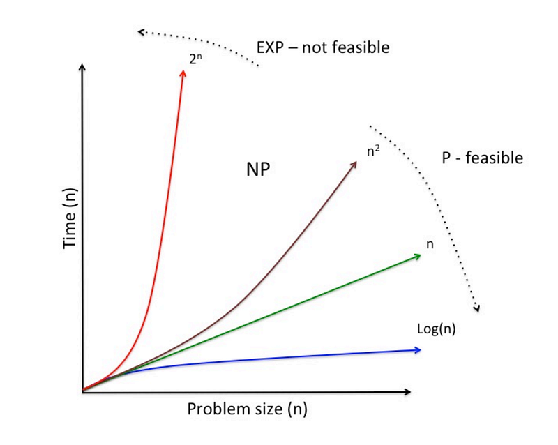
Source: cnbeta.com | A chart describing the different categories of algorithmic efficiency using Big O Notation.

Exponential algorithms (“EXP” algorithms, as in the chart above) are incredibly inefficient and impractical for large quantities of data, as the computation time required is massive. However, it’s still not a bad option for use cases where a very small amount of input data is required.

On the other hand, Polynomial algorithms (“P” algorithms, as in the chart above) are efficient and practical ways to compute various problems, in comparison to their Exponential counterpart.

“Now wait”, you might be saying to yourself. “Why are we comparing the efficiency of algorithms rather than the computer themselves”?

Well, while we claim that both machines are Universal Turing-complete, the reality is that you may not be able to take advantage of the characteristics of a UTM for every problem that you run on these computers! Rather, this depends on the algorithm you are using to solve the problem — whether it’s taking advantage of the UTM-like characteristics that the machine possesses. This explains why we need to talk about this here, and emphasizes why algorithm development is such a key cornerstone in developing more efficient methods of computation.

Wouldn’t it be great if there was a way to reduce the complexity of an exponential algorithm to a polynomial one? Or even better, come up with new algorithms that could compute the same task more efficiently?

Well as it turns out, scientists have been inventing new, more efficient algorithms to compute various kinds of complex problems for years! A great example of this is Shor’s Algorithm, which promises to be able to factor numbers, a problem only solvable in exponential time, in polynomial time!

The only problem is that algorithms like Shor’s can’t be run on our regular computers. We need a special kind of computer, one that produces non-deterministic results to help us out.

But wait, is that even possible? How can anything produce truly non-deterministic results?

Let’s talk about Quantum Computers, and what makes them so special!

Quantum Computing

The world of tiny, sub-atomic particles is quite interesting. Not just because of their small size, but because of their completely non-intuitive properties that you don’t find anywhere else in nature.

Quantum Computing relies on quantum mechanical properties, such as superposition and entanglement to allow for performing highly parallel computations and solving specific problems much faster and/or more accurately than classical computers can.

These non-intuitive properties allow for non-deterministic computation, where the task of the algorithm and the algorithm designer is to manipulate probabilities in such a way that the user obtains the desired results, often without knowing what those results should be or what they look like.

The aim for developing quantum algorithms is two-fold: being able to manipulate a system’s probabilities to be able to yield desirable outcomes, and demonstrating a distinct advantage over classical computers in that particular application. Of course, this is easier said than done and remains a formidable challenge in the field today.

Essentially, what Quantum Computers represent is a UTM that can take an input state such as a Turing machine, and produce several possible output states.

“But wait”, some of you might be saying. “That isn’t even a valid mathematical function!”. And you’d be right.

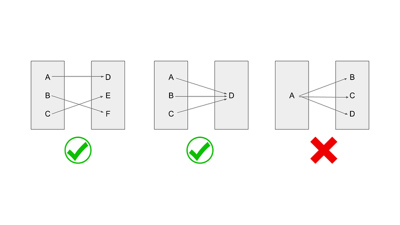
An image depicting the different kinds of mathematical functions

For those who don’t know, functions are simply a mapping of an input to an output. Imagine a computer that outputs a unique answer for every possible input. That is a One-One function.

A function that outputs one answer for every possible input is called a Many-One function.

But how about a One-Many function? Well, turns out that in mathematics, such a function is invalid, meaning that it isn’t a real function!

For the longest time, it was believed that a computing machine that worked on the principle of such One-Many functions was impossible. That is, until Quantum Computers and DNA Computers rolled around, demonstrating the existence of such a computational model.

This kind of UTM is called a NUTM: a Non-deterministic Universal Turing Machine.

The best explanation for such a phenomenon is a concept called Serendipity.

This is when a computer is able to correctly guess which of the output states to choose so as to reach the goal state the fastest for each state.

Clearly, this phenomenon seems “magical”, “hypothetical” and even “fictitious” — but it’s not! And that, in my opinion, is what makes NUTMs so beautiful ❤️

Before we move on, remember how I alluded to DNA Computers having a bit of a twist as well? Well, as it turns out, DNA Computers are capable of performing non-deterministic computations as well!

But wait, how is a DNA computer’s hybridization process for solving the Traveling Salesman Problem a non-deterministic computation? Well, it isn’t!

The TSP is not a non-deterministic algorithm. However, other algorithms that actually are non-deterministic can be executed on a DNA Computer as well by encoding nucleotides as Thue Strings.

This means that DNA Computers can perform parallel computations, while still having the capability to perform non-deterministic computations if necessary.

I’ll be talking about this in-depth in a future article, but for now, all you need to know is that non-deterministic computation is possible using DNA Computers. Just trust me on that one 🤞

So, is this the end for Quantum Computers?

NOPE!

Let me explain.

There’s no doubt that as far as the TSP is concerned, algorithmically the DNA Computer would be way more convenient to use as you don’t have to design algorithms that manipulate probabilities to get to the right result. They can instead function more like classical computers, possibly allowing for existing hardware to be integrated efficiently as well.

The word to highlight here is “algorithmically”. Practically speaking, the hardware that could allow DNA Computing to revolutionize the world is nowhere near ready. In comparison, Quantum Computers are a lot more capable of tackling such problems. Even though there are still a bunch of engineering challenges left to solve, they are a lot more capable than DNA Computers at the time of publishing this article.

I have identified four key guidelines for choosing the kind of computer that would be most suitable for a particular task. They are:

• the nature of the problem to be solved,
• the selection of the most suitable algorithm for the task,
• the existence of a suitable platform,
• and the practical feasibility of implementing the solution on the chosen platform.

Let’s start off with the first guideline. If you are trying to solve a problem like 31+65, you obviously don’t need some gargantuan supercomputer to do that for you. A simple calculator would suffice. Maybe you don’t even need one if you’re used to doing math sums in your head.

The nature of such a problem is so simple that even the most basic methods would suffice.

However, let’s assume that you need to find the factors of a 300-digit number — something like this:

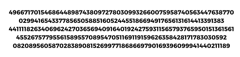
An image of a 300-digit number

As discussed previously, finding the factors of a number is a very difficult problem. Such a problem cannot be solved using a typical calculator, and especially not your own mind. The hardware is simply incapable, as well as the algorithms being used on it.

Shor’s algorithm promises to solve this problem in a much more efficient way using an incredibly novel approach. This brings us to the second guideline, as it is currently the most suitable algorithm for the task at hand.

However, this algorithm cannot be run on the classical hardware that you and I use today. The third guideline requires us to have a platform that can support Shor’s algorithm, which must operate in a fundamentally different from classical computers.

That platform happens to be Quantum Computers, which possess the characteristics required to run Shor’s algorithm, thereby finding the factors of this 300-digit number.

It’s important to note that while a particular computing platform may be more capable than another, solutions on a particular platform might come around more intuitively to the scientists developing the algorithms. In the case of Shor for example, the theoretical concept of quantum computers is what really enabled him to be able to come up with the algorithm in the first place.

Now, we’re still left with the fourth and final guideline, which is currently where we’re stuck. Quantum Computers may have the theoretical capability to support Shor’s algorithm, but there are still a ton of engineering challenges to overcome to be able to demonstrate this practically.

Quantum Computers are highly error-prone, don’t have efficient methods for correcting said errors, and lack the number of qubits (quantum bits) required to execute this algorithm at the required scale.

I believe that in the end, it’s not a matter of whether one technology will replace the other, but rather recognizing that both DNA Computing and Quantum Computing have their practical differences, leading to various strengths and limitations when implementing a particular algorithm.

A great example of this is how Quantum Computers can increase their state space by 2^N, where N represents the number of qubits in the system. In comparison, the pairing of DNA strands that happens in DNA Computers during the Hybridization process is both physical and isn’t exponential in nature.

This may very well affect the kinds of algorithms that can be developed for DNA Computers, and how they’re executed on the physical hardware.

I’ll be publishing an article soon that details newer methods for DNA Computation, referencing the same paper as well. Follow me to stay tuned :)

PS: Would appreciate some feedback on the article! Do leave a comment letting me know what you think 👇👇